
This case study details how a shift from traditional agile metrics (Story Points, Velocity) to actionable flow metrics (Work In Progress, Cycle Time, Throughput) reduced Cycle Times, increased quality, and increased overall predictability at Siemens Health Services. Moving to a continuous flow model augmented Siemens’ agility and explains how predictability is a systemic behavior that one has to manage by understanding and acting in accordance with the assumptions of Little’s Law and the impacts of resource utilization.
1. INTRODUCTION
Siemens Health Services provides sophisticated software for the Healthcare industry. We had been using traditional “agile” metrics (e.g. story points, velocity) for several years, but never realized the transparency and predictability that those metrics promised. By moving to the simpler, more actionable metrics of flow (work in progress, Cycle Time, and throughput) we were able to achieve a 42% reduction in Cycle Time and a very significant improvement in operational efficiency. Furthermore, adopting Kanban has led to real improvements in quality and collaboration, all of which have been sustained across multiple releases. This article describes how moving to a continuous flow model augmented Siemens’ agility and explains how predictability is a systemic behavior that one has to manage by understanding and acting in accordance with the assumptions of Little’s Law and the impacts of resource utilization.
Before reading further, please note that we assume the reader is familiar with Kanban and its underlying principles of pull (limiting work in progress), and flow. No attempt will be made to explain these concepts in any detail.
2. BACKGROUND
Siemens Health Services (HS), the health IT business unit of Siemens Healthcare, is a global provider of enterprise healthcare information technology solutions. Our customers are hospitals and large physician group practices. We also provide related services such as software installation, hosting, integration, and business process outsourcing.
The development organization for Siemens HS is known as Product Lifecycle Management (PLM) and consists of approximately 50 teams based primarily in Malvern, Pennsylvania, with sizable development resources located in India and Europe. In 2003 the company undertook a highly ambitious initiative to develop Soarian®, a brand new suite of healthcare enterprise solutions.
The healthcare domain is extremely complex, undergoing constant change, restructuring, and regulation. It should be of no surprise that given our domain, the quality of our products is of the highest priority; in fact, one might say that quality is mission critical. Furthermore, the solutions we build have to scale from small and medium sized community hospitals to the largest multi-‐facility healthcare systems in the world. We need to provide world-‐class performance and adhere to FDA, ISO, Sarbanes–Oxley, patient safety, auditability, and reporting regulations.
Our key business challenge is to rapidly develop functionality to compete against mature systems already in the market. Our systems provide new capabilities based on new technology that helps us to leapfrog the competition. In this vein, we adopted agile development methodology, and more specifically Scrum/XP practices as the key vehicles to achieve this goal.
Our development teams transitioned to agile in 2005. Engaging many of the most well-‐known experts and coaches in the community, we undertook an accelerated approach to absorbing and incorporating new practices. We saw significant improvement over our previous waterfall methods almost immediately and our enthusiasm for agile continued to grow. By September 2011 we had a mature agile development program, having adopted most Scrum and XP practices.
Our Scrum teams included all roles (product owners, scrum masters, business analysts, developers and testers). We had a mature product backlog and ran 30-‐day sprints with formal sprint planning, reviews, and retrospectives. We were releasing large batches of new features and enhancements once a year (mostly because that’s the frequency at which we’ve always released). Practices such as continuous integration (CI), test-‐driven development (TDD), story-‐driven development, continuous customer interaction, pair programming, planning poker, and relative point-‐based estimation were for the most part well integrated into our teams and process. Our experience showed that Scrum and agile practices vastly improved collaboration across roles, improved customer functionality, improved code quality and speed. Our Scrum process includes all analysis, development and testing of features. A feature is declared “done” only after it has passed validation testing in a fully integrated environment performed by a Test Engineer within each Scrum Team. Once all release features are complete, Siemens performs another round of regression testing, followed by customer beta testing before declaring general availability and shipping to all our customers.
2.1 The Problem
Despite many improvements and real benefits realized by our agile adoption, our overall success was limited. We were continually challenged to estimate and deliver on committed release dates. Meeting regulatory requirements and customer expectations require a high degree of certainty and predictability. Our internal decision checkpoints and quality gates required firm commitments. Our commitment to customers, internal stakeholder expectations and revenue forecasts required accurate release scope and delivery forecasts that carry a very high premium for delay.
At the program and team levels, sprint and release deadlines were characterized by schedule pressure often requiring overtime and the metrics we collected were not providing the transparency needed to clearly gauge completion dates or provide actionable insight into the state of our teams.
In the trenches, our teams were also challenged to plan and complete stories in time-‐boxed sprint increments. The last week of each sprint was always a mad rush by teams to claim as many points as possible, resulting in hasty and over-‐burdened story testing. While velocity rates at sprint reviews often seemed good, reality pointed to a large number of stories blocked or incomplete and multiple features in progress with few, if any, features completing until the end of the release. This incongruity between velocity (number of points completed in a sprint) and reality, was primarily caused by teams starting too many features and/or stories. It had been common practice to start multiple features at one time to mitigate possible risks. In addition, whenever a story or feature was blocked (for a variety of reasons such as waiting for a dependency from another team, waiting for customer validation, inability to test because of environmental or build break issues, etc.), teams would simply start the next story or feature so that we could claim the points which we had committed to achieve. So, while velocity burn-‐ups could look in line with expectations, multiple features were not being completed on any regular cadence, leading to bottlenecks especially at the end of the release as the teams strove to complete and test features. During this period we operated under the assumption that if we mastered agile practices, planned better, and worked harder we would be successful. Heroic efforts were expected.
2.2 Why Kanban
In November of 2011 executive management chartered a small team of director level managers to coordinate and drive process improvement across the PLM organization, with the key goal of finally realizing the predictability, operational efficiency, and quality gains originally promised by our agile approach. After some research, the team concluded that any changes had to be systemic. Other previous process improvements had focused on specific functional areas such as coding or testing, and had not led to real improvements across the whole system or value stream. By value stream in this context we mean all development activities performed within the Scrum Teams from “specifying to done”. By reviewing the value stream with a “Lean” perspective we realized that our problems were indeed systemic, caused by our predilection for large batch sizes such as large feature releases. Reading Goldratt (Goldratt, 2004), and Reinertsen (Reinertsen, 2009) we also came to understand the impacts of large, systemic queues. Coming to the understanding that the overtime, for which programmers were sacrificing their weekends, may actually have been elongating the release completion date was an epiphany.
This path inevitably led us to learn about Kanban. We saw in Kanban a means of enforcing Lean and continuous improvement across the system while still maintaining our core agile development practices. Kanban would manage Work in Progress, Cycle Time, and Throughput by providing a pull system and thus reduce the negative impacts of large batches and high capacity utilization. Furthermore, we saw in Kanban thepotential for metrics that were both tangible (and could be well understood by all corporate stake-‐holders) and provide individual teams and program management with data that is highly transparent and actionable.
We chose our revenue-‐cycle application as our pilot, consisting of 15 scrum teams located in Malvern, PA., Brooklyn, N.Y., and Kolkata, India. Although each scrum team focuses on specific business domains, the application itself requires integrating all these domains into a single unitary customer solution. At this scale of systemic complexity, dependency management, and continuous integration, a very high degree of consistency and cohesion across the whole program is required. With this in mind, we designed a “big-‐bang” approach with a high degree of policy, work-‐unit, workflow, doneness, and metric standardization across all teams. We also concluded that we needed electronic boards: large monitors displayed in each team room that would be accessible in real time to all our local and offshore developers. An electronic board would also provide an enterprise management view across the program and a mechanism for real-‐time metrics collection.
Our initial product release using Kanban began in April 2012 and was completed that December. Results from our first experience using Kanban were far better than any of our previous releases. Our Cycle Time looked predictable and defects were down significantly.
Our second release began in March 2013 and finished in September of that same year. We continue to use Kanban for our product development today. As we had hoped, learnings and experience from the first release led to even better results in the releases that followed.
3. ACTIONABLE METRICS
Now that we had decided to do Kanban at Siemens HS, we had to change the metrics we used so that we could more readily align with our newfound emphasis on flow. The metrics of flow are very different than traditional scrum-‐style metrics. As mentioned earlier, instead of focusing on things like story points and velocity, our teams now paid attention to Work in Progress (WIP), Cycle Time, and Throughput. The reason these flow metrics are preferable to traditional agile metrics is because they are much more actionable and transparent. By transparent we mean that the metrics provide a high degree of visibility into the teams’ (and programs’) progress. By actionable, we mean that the metrics themselves will suggest the specific team interventions needed to improve the overall performance of the process.
To understand how flow metrics might suggest improvement interventions we must first explore some definitions. For Siemens HS, we defined WIP to be any work item (e.g. user story, defect, etc.) that was between the “Specifying Active” step and the “Done” step in our workflow (see Figure 1).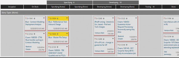
Figure 1. Example Kanban Board
Cycle Time was defined to be the amount of total elapsed time needed for a work item to get from “Specifying Active” to “Done”. Throughput was defined as the number of work items that entered the “Done” step per unit of time (e.g. user stories per week). It is important to note here that Throughput is subtly different than velocity. With velocity, a team measures story points per iteration. With Throughput, a team simply counts the number of work items completed per arbitrary unit of time. That unit of time could be days, weeks, months— or even iterations.
It is one of those interesting quirks of fate that these three metrics of flow—WIP, Cycle Time, and Throughput—are inextricably linked through a simple yet powerful relationship known as Little’s Law (Little, 2011) as shown in Figure 2:

Figure 2. Little’s Law
That is to say, change in any one of these metrics will almost certainly cause a change in one or both of the others. If any one of these metrics are not where we want it to be, then this relationship tells us exactly what lever(s) to pull in order to correct. In short, Little’s Law is what makes the metrics of flow actionable.
Think about how profound this relationship is for a second. Little’s Law tells us most (not all) we need to know about the relationship between WIP and Cycle Time. Specifically, for the purposes of this paper, Little’s Law formalizes the fact that—assuming certain assumptions are met—a decrease in average WIP will lead to a decrease in average Cycle Time. To affect positive change in your overall process, you don’t need to go through a complex agile transformation, you don’t need to do more intense estimation and planning. For the most part, all you need to do is control the number of things that you are working on at any given time. Simple, but true.
A full discussion of Little’s Law is well beyond the scope of this article (for a fuller—though still not complete—treatment of Little’s Law, please see the References and Appendix A at the end of this paper). The point of mentioning it here is to raise awareness to relationship of these crucial metrics. Most agile teams don’t look at WIP, Cycle Time, and Throughput; yet it is the understanding of these metrics and how they affect one another that is the key to taking an actionable approach to agile management. The rest of this article will explain such an approach.
1. Types of Chart
The two main types of charts we used to visualize these metrics were the Cumulative Flow Diagram (CFD) and the Cycle Time Scatterplot. As was the case with Little’s Law, a deep discussion around what these charts are and how to interpret them is well beyond the scope of this article. We encourage you to do some investigation into these charts on your own as they are among the best tools out there for managing flow. Unfortunately, however, there is a lot of misinformation and disinformation floating around about how these charts work; therefore, we have included some links to resources that you may find useful in the references section at the end of this article.
2. Process Performance before Kanban
We have stressed throughout this paper that predictability is of paramount importance to Siemens HS. So how was the organization doing before Kanban?Figure 3 is a scatterplot of Cycle Times for finished stories in the Financials organization for the whole release before Kanban was introduced.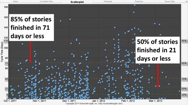
Figure 3. Cycle Times in the release before Kanban
What this scatterplot tells us is that in this release, 50% of all stories finished in 21 days or less. But remember we told you earlier that Siemens HS was running 30-‐day sprints? That means that any story that started at the beginning of a sprint had little better than 50% chance of finishing within the sprint. Furthermore, 85% of stories were finishing in 71 days or less—that’s 2.5 sprints! What’s worse is that Figure 3 shows us that over the course of the release the general trend of story Cycle Times was getting longer and longer and longer (see Figure 4).
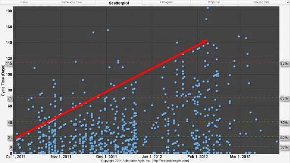
Figure 4. General Upward Trend of Cycle Times before the Introduction of Kanban
Figure 4 is not a picture of a very predictable process.
So what was going on here? A simplified interpretation of Little’s Law tells us that if Cycle Times are too long, then we essentially have two options: decrease WIP or increase Throughput. Most managers inexplicably usually opt for the latter. They make teams work longer hours (stay late) each day. They make teams work mandatory weekends. They try to steal resources from other projects. Some companies may even go so far as to hire temporary or permanent staff. The problem with trying to impact Throughput in these ways is that most organizations actually end up increasing WIP faster than they increase Throughput. If we refer back to Little’s Law, we know that if WIP increases faster than Throughput, then Cycle Times will only increase. Increasing WIP faster than increasing Throughput only exacerbates the problem of long Cycle Times.
3. How We Learned to Reduce Cycle Time
Our choice (eventually) was the much more sensible and economical one: reduce Cycle Times by limiting WIP through the use of Kanban. What most people fail to realize is that limiting WIP can be as simple as making sure that work is not started at a faster rate than work is completed (please see Figure 5 as an example of how mismatched arrival and departure rates increases WIP in the process). Matching arrival rates to departure rates is the necessary first step to stabilizing a system. Only by operating a stable system could we hope to achieve our goal of predictability.Unfortunately for us, however, the first release that we implemented Kanban, we chose not to limit WIP right away (the argument could be made that we weren’t actually doing “Kanban” at that point). Why? Because early on in our Kanban adoption the teams and management resisted the imposition of WIP limits. This was not unexpected, as mandating limits on work went against the grain of the then current beliefs. We therefore decided to delay implementing WIP limits until the third month of the release. This allowed the teams and management to gain a better familiarity of the method and become more amenable.The delay in implementing WIP limits cost us and in retrospect we should have pushed harder to impose WIP limits from the outset. As you might expect, because of the lack of WIP limits, the very same problems that we saw in the previous release (pre-‐Kanban) started to appear: Cycle Times were too long and the general trend was that they were getting longer.Taking a look at the CFD (Figure 5) in the first release with Kanban clearly shows how our teams were starting to work on items at a faster rate than we were finishing them.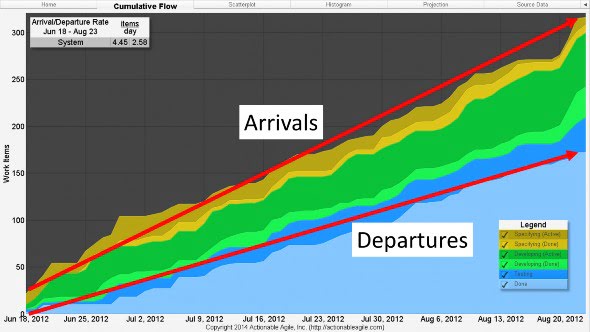
Figure 5. CFD Early on in the first release with Kanban
This disregard for when new work should be started resulted in an inevitable increase in WIP which, in turn, manifested itself in longer Cycle Times (as shown in Figure 6).
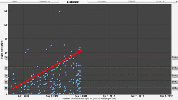
Figure 6. Scatterplot early on in the first release with Kanban
Upon seeing these patterns emerge, we instituted a policy of limiting WIP across all teams. Limiting WIP had the almost immediate effect of stabilizing the system such that Cycle Times no longer continued to grow (as shown in Figure 7).
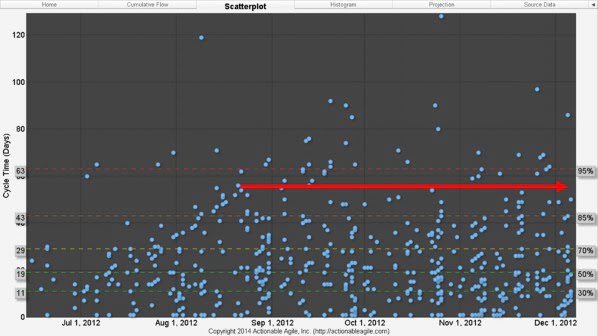
Figure 7. Stabilized Cycle Times after introducing WIP Limits
Over the course of our first release with Kanban, the 85th percentile of story Cycle Time had dropped from 71 days to 43 days. And, as you can see from comparing Figure 4 to Figure 7 (the release before Kanban, and the first release using Kanban, respectively) the teams were suffering from much less variability. Less variability resulted in more predictability. In other words, once we limited WIP in early September 2012, Cycle Times did not increase indefinitely as they did the release before. They reached a stable state at about 41 days almost immediately, and stayed at that stable state for the rest of the release.
This stabilization effect of limiting WIP is also powerfully demonstrated in the CFD (Figure 8):
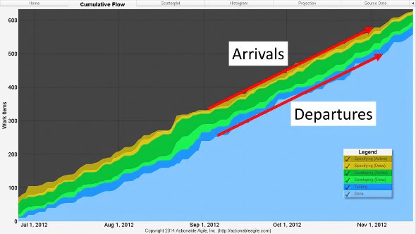
Figure 8. CFD in the first release with Kanban after WIP limits were introduced
The second release after the introduction of Kanban saw much the same result (with regard to predictability). 85 percent of stories were finishing within 41 days and variability was still better controlled. Looking at the two scatterplots side by side bears this out (Figure 9).
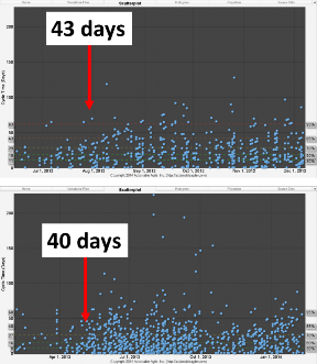
Figure 9. Scatterplots of the first release using Kanban (above) and the second release of Kanban (below)
Hopefully it is obvious to the reader that by taking action on the metrics that had been provided; we had achieved our goal of predictability. As shown in Figure 9, our first release using Kanban yielded Cycle Times of 43 days or less, and our second release using Kanban yielded Cycle Times of 40 days or less. This result is the very definition of predictability.
By attaining predictable and stable Cycle Times we would now be able to use these metrics as input to future projections. These shorter Cycle Times and decreased variability also led to a tremendous increase in quality. Figure 10 shows how Kanban both reduced the number of defects created during release development well as minimizing the gap between defects created and defects resolved during the release.
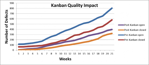
Figure 10. Quality compared between releases
By managing queues, limiting work-‐in progress and batch sizes and building a cadence through a pull system (limited WIP) versus push system (non-‐limited WIP) we were able to expose more defects and execute more timely resolutions. On the other hand “pushing” a large batch of requirements and/or starting too many requirements delays discovery of defects and other issues; as defects are hidden in incomplete requirements and code.
By understanding Little’s Law, and by looking at how the flow appears in charts like CFDs and scatterplots, Siemens HS could see what interventions were necessary to get control of their system. Namely, the organization was suffering from too much WIP, which was, in turn, affecting Cycle Time and quality. In taking the action to limit WIP, Siemens saw an immediate decrease in Cycle Time and an immediate increase in quality.
These metrics also highlighted problems within the Siemens HS product development process, and the next section will discuss what next steps the organization is going to implement in order to continue to improve its system.
4. HOW METRICS CHANGED EVERYTHING
Apart from the improvements in predictability and quality, we also saw significant improvements in operational efficiency. We had “real-‐time” insight into systemic blocks, variability and bottlenecks and could take appropriate actions quickly. In one case by analyzing Throughput (story run rate) and Cycle Time for each column (specifying, testing and developing), we were able to clearly see where we were experiencing capacity problems. We were also able to gauge our “flow efficiency” by calculating the percentage of time stories were being worked on or “touched” versus “waiting” or “blocked”. Wait time is the time a story sits in an inactive or done queue because moving to the next active state is prevented by WIP limits. Blocked time is the time that work on a story is impeded, including impediments such as build-‐breaks, defects, waiting for customer validation etc. The calculation is made by capturing time spent in the “specifying done and developing done” column plus any additional blocked time, which we call “wait time”. (Blocked or impediment data is provided directly by the tool we are using). Subtracting “wait time” from total Cycle Time gives us “touched time”. Calculating flow efficiency is simply calculating the percentage of total touch time over total Cycle Time. Flow efficiency percentage can act as a powerful Key Performance Indicator (KPI) or benchmark in terms of measuring overall system efficiency.
This level of transparency, broadly across the program and more deeply within each team enabled us to make very timely adjustments. Cumulative flow diagrams provided a full picture at the individual team and program levels where our capacity weaknesses lay and revealed where we needed to make adjustments to improve Throughput and efficiency. For example, at the enterprise level using the cumulative flow diagram the management team was able to see higher Throughput in “developing” versus “testing” across all teams and thus make a decision to invest in increasing test automation exponentially to re-‐balance capacity. This was actually easy to spot as the “developing done” state on the CFD consistently had stories queued up waiting for the “testing” column WIP limits to allow them to move into “testing”.
At the team level, the metrics would be used to manage WIP by adjusting WIP limits when needed to ensure flow and prevent the build-‐up of bottlenecks and used extensively in retrospectives to look at variability. By using the scatterplot, teams could clearly see stories whose cycle time exceeded normal ranges, perform root cause analysis and take steps and actions to prevent recurrence. The CFD also allowed us to track our average Throughput or departure-‐rate (the number of stories we were completing per day/week etc.) and calculate an end date based on the number of stories remaining in the backlog – (similar to the way one uses points and velocity, but more tangible). Furthermore, by controlling WIP and managing flow we saw continued clean builds in our continuous integration process, leading to stable testing environments, and the clearing of previously persistent testing bottlenecks.
The results from the first release using Kanban were better than expected. The release completed on schedule and below budget by over 10%. The second release was even better: along with sustained improvements in Cycle Time, we also became much faster. By reducing Cycle Time we were increasing Throughput, enabling us to complete 33% more stories than we had in the previous release, with even better quality in terms of number of defects and first pass yield – meaning the percentage of formal integration and regression tests passing the first time they are executed. In the release prior to Kanban our first pass yield percentage was at 75%, whereas in the first Kanban release the pass percentage rose to 86% and reached 95% in our second release using Kanban.
The metrics also gave us a new direction in terms of release forecasting. By using historical Cycle Times we could perform Monte-‐Carlo simulation modelling (Magennis, 2012) to provide likely completion date forecasts. If these forecasts proved reliable, we would no longer need to estimate. In our second Kanban release we adopted this practice along with our current points and velocity estimation planning methods and comparedthe results. Apart from the obvious difference in the use of metrics versus estimated points, the simulation provides a distribution of likely completion timeframes instead of an average velocity linear based forecast – such as a burn up chart. Likewise Cycle Time metrics are not based on an average (such as average number of points) but on distributions of actual Cycle Times. The histogram shown below in Figure 11 is an example of actual historical Cycle Time distributions that Siemens uses as input to the modelling tool. In this example 30% of stories accounting for 410 actual stories had Cycle Times of 9 days or less, the next 20% accounting for 225 stories had cycle-‐times of 10 to 16 days, and so forth.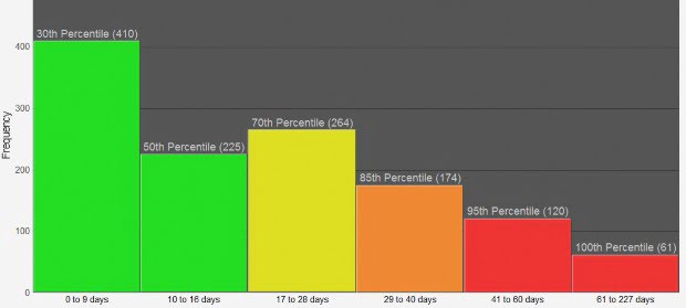
Figure 11. Cycle Time Distributions
What we learned was that velocity forecasts attempt to apply a deterministic methodology to an inherently uncertain problem. That type of approach never works. By using the range or distributions of historical Cycle Times from the best to worst cases and simulating the project hundreds of times, the modelling simulation provides a range of probabilistic completion dates at different percentiles. For example, see figure 11 below showing likely completion date forecasts used in release planning. Our practice is to commit to the date which is closest to the 85th percent likelihood as is highlighted in the chart. As the chart shows we are also able to use the model to calculate likely costs at each percentile.
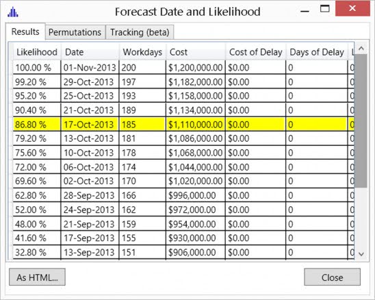
Figure 12. Result of Monte-‐Carlo simulation showing probability forecast at different percentages
Over the course of the release the model proved extremely predictive; moreover, it also provided to Siemens the ability to perform ongoing risk analysis and “what-‐if” scenarios with highly instructive and reliable results. For example, in one case, to meet an unexpected large scope increase on one of the teams, the Program Management Team was planning to add two new Programmers. The modelling tool pointed to adding a Tester to the team rather than adding programming. The tool proved very accurate in terms of recommending the right staffing capacity to successfully address this scope increase.
At the end of the day, it was an easy decision to discard story point velocity-‐based estimation and move to release completion date forecasts. The collection of historical Cycle Time metrics that were stable and predictable enabled Siemens to perform Monte-‐Carlo simulations, which provided far more accurate and realistic release delivery forecasts. Thus a huge gap in our agile adoption closed. In analyzing the metrics, Siemens also discovered that there was no correlation between story point estimates and actual Cycle Time.
Siemens also gained the ability to more accurately track costs; as we discovered that we could in fact correlate Cycle Time to actual budgetary allocations. Siemens could now definitively calculate the unit costs of a story, feature and/or a release. By using the modelling tool we could now forecast likely costs along with dates. Moreover, we could put an accurate dollar value on reductions or increases in Cycle Times.
The metrics also improved communication with key non-‐PLM stakeholders. It had always been difficult translating relative story points to corporate stakeholders who were always looking for time based answers and who found our responses based on relative story points confusing. Metrics such as Cycle Time and Throughput are very tangible and especially familiar in a company such as Siemens with a large manufacturing sector.
Implementing Kanban also had a positive impact on employee morale. Within the first month, scrum-‐ masters reported more meaningful stand-‐ups. This sentiment was especially expressed and emphasized by our offshore colleagues, who now felt a much higher sense of inclusion during the stand-‐up. Having the same board and visualization in front of everyone made a huge difference on those long distant conference calls between colleagues in diametrically opposed time zones. While there was some skepticism as expected,
overall comments from the teams were positive; people liked it. This was confirmed in an anonymous survey we did four months into the first release that we used Kanban: the results and comments from employees were overwhelmingly positive. Furthermore, as we now understood the impact of WIP and systemic variability, there was less blame on performance and skills of the team. The root of our problem lay not in our people or skills, but in the amount of Work in Progress (WIP).
5. CONCLUSIONS AND KEY LEARNINGS
Kanban augmented and strengthened our key Agile practices such as cross-‐functional scrum teams, story driven development, continuous integration testing, TDD, and most others. It has also opened the way to even greater agility through our current plan to transition to continuous delivery.
Traditional agile metrics had failed Siemens HS in that they did not provide the level of transparency required to manage software product development at this scale. Looking at a burn-‐down chart showing average velocity does not scale to this level of complexity and risk. This had been a huge gap in our agile adoption, which was now solved.
Understanding flow—and more importantly the metrics of flow—allowed Siemens to take specific action in order improve overall predictability and process performance. On this note, the biggest learning was understanding that predictability was a systemic behavior that one has to manage by understanding and acting in accordance with the assumptions of Little’s law and the impacts of resource utilization.
Achieving a stable and predictable system can be extremely powerful. Once you reach a highly predictable state by aligning capacity and demand, you are able to see the levers to address systemic bottlenecks and other unintended variability. Continuous improvement in a system that is unstable always runs the risk of improvement initiatives that result in sub-‐optimizations.
The extent of the improvement we achieved in terms of overall defect rates was better than expected. Along with the gains we achieved through managing WIP, we had placed significant focus on reinforcing and improving our CI and quality management practices. Each column had its own doneness criteria and by incorporating “doneness procedures” into our explicit policies we were able to ensure that all quality steps were followed before moving a story to the next column – for example moving a story from “Specifying” to “Developing”. Most of these practices had predated Kanban; however the Kanban method provided more visibility and rigor.
The metrics also magnified the need for further improvement steps: The current Kanban implementation incorporates activities owned within the Scrum Teams; but does not extend to the “backend process” — regression testing, beta testing, hosting, and customer implementation. Like many large companies Siemens continues to maintain a large batch release regression and beta testing process. Thus begging the question, what if we extended Kanban across the whole value stream from inception to implementation at the customer? Through the metrics, visualization, managing WIP and continuous delivery we could deliver value to our customers faster and with high quality. We could take advantage of Kanban to manage flow, drive predictable customer outcomes, identify bottlenecks and drive lean continuous improvement through the testing, operations and implementation areas as well. In late 2013 we began our current and very ambitious journey to extend the Kanban method across the whole value stream.
Finally it is important to say that Kanban has had a very positive impact on employee morale. It has been embraced across all our teams in all locations without exception and has improved collaboration. Furthermore the use of metrics instead of estimation for forecasting has eliminated the emotion and recrimination associated with estimation. Anyone wishing to go back to sprinting would be few and far between, including even those who had previously been the most skeptical.
ACKNOWLEDGEMENTS
We would like to thank the Agile Alliance and especially Rebecca Wirfs‐Brock for the invitation to share our experiences. We would also like to thank Siemens HS for allowing us to publish this case study. Last, but certainly not least, we would like to thank Nanette Brown for her tireless efforts in guiding us through this process. This article would not have come together without her keen insights, questions, and edits. Thanks, Nanette, we couldn’t have done it without you!
APPENDIX A: A VERY SHORT INTRODUCTION TO LITTLE’S LAW FOR AGILE TEAMS
When most lean-‐agile adherents talk about Little’s Law, we usually state it in terms of the Throughput (or the departure rate) of a system as shown here:
Cycle Time = Work-In-Progress / Throughput (1)
where Throughput is the average departure rate of the system (or the average output of a production process per unit time), Work in Progress is the amount of inventory between the start and end points of a process, and Cycle Time is the time difference between when a piece of work enters the system and when it exits the system. Cycle Time can also be thought of as “flow time” in the Kanban context (or it can be thought of as the amount a time a unit of work spends as Work in Progress).
I wonder how many people know, however, that this is not the original “version” of the law. When first written down (sometime in the 1950s—and subsequently “proved” in 1961) the law was actually defined in terms of the arrival rate of a system (not the departure rate). That definition generally looked something like:
L = λ* W (2)
- Where, L = average number of items in the queuing system,
- W = average waiting time in the system for an item, and
- λ = average number of items arriving per unit time
For this law to hold when stated in terms of arrival rate, at least two things need to be true: first, we must have some notion of system stability; and second, the calculation must be done using consistent units. Simple enough.
Or is it?
When Little’s Law is usurped for use in Lean applications, equation (1) is often stated by so-‐called experts to justify a reduction of WIP as a means to reduce Cycle Time. Then some wild flailing of the hands and some clearing of the throat is made along with some barely-‐audible mention of system stability (if it is mentioned at all and not swept under the rug entirely). The “experts” then quickly move on to the next topic so as to avoid any embarrassing questions as to what “system stability” really means.
It is a fairly straightforward exercise (and one I leave up to the reader) to demonstrate that equations (1) and (2) are logically equivalent. What is not so straightforward is to understand in what situations equation is applicable given that (1) is stated in terms of departure rate and (2) is stated in terms of arrival rate (do we even need to state different assumptions for the two forms of the equation?).It turns out that when talking about Little’s Law in the form of equation (1), five conditions must exist in order for the law to be valid (for the purposes of this discussion, I’m going to assume that the total WIP in a candidate process never goes to zero—as should normally be the case in most good Kanban systems):
- The average output or departure rate (Throughput) should equal the average input or arrival rate (λ)
- All work that is started will eventually be completed and exit the system.
- The amount of WIP should be roughly the same at the beginning and at the end of the time interval chosen for the calculation.
- The average age of the WIP is neither growing nor declining.
- The calculation must be performed using consistent units.
What’s most interesting to me about what’s stated here is what’s not stated here. There is no mention of characteristic statistical distributions of arrival or departure rates, there is no mention of all work items being of equal (or roughly equal) size, and there is no mention of a specific queuing discipline—to name just a few.
When these five conditions are met, Little’s Law is exact. Period. That’s a pretty bold statement, but it’s true nonetheless. One thing to note about exactness is that Little’s Law is only exact after the fact. Little’s Law cannot be used to make deterministic predictions about the future. For example, let’s say that for the past six months you have had an average of 12 items in progress and an average Throughput of 4 items per week, which gave you an average Cycle Time of 3 weeks per item. Now let’s say you want to reduce your Cycle Time to 2 weeks. Simple, right? Just lower WIP to an average of 8 items and Little’s Law predicts your Cycle Time
will magically lower to 2 weeks. Wrong. Little’s Law will not guarantee this outcome. That is to say, that Little’s Law does not guarantee that lowering WIP will have a deterministic effect on Cycle Time.
So why learn about Little’s Law? The proper application of Little’s Law is not a deterministic one. It is understanding the assumptions behind the law that make it work (as stated above). Using those assumptions as a template for your own process policies is what will make your process predictable. Implementing those policies is what makes flow metrics (WIP, Cycle Time, and Throughput) truly actionable.
REFERENCES
Goldratt, Eliyahu M. “The Goal, A Process of Ongoing Improvement” North River Press, 3rd revised edition, 2004
Little, John D C “Little’s Law as Viewed on its 50th Anniversary” Operations Research, Vol. 59, No. 3, May–June 2011, pp. 536–549 Magennis, Troy “Forecasting and Simulating Software Development Projects – Effective Modeling of Kanban & Scrum projects using Monte-‐Carlo Simulation” self-‐published 2011
Reinertsen, Donald G. “The Principles of Product Development FLOW” Celeritas Publishing, 2009 Vacanti, Daniel, Corporate Kanban blog, http://www.corporatekanban.com
The Cumulative Flow Diagrams and Scatterplots have been created courtesy of Actionable Agile, Inc. (http://www.actionableagile.com)